Metropolis-Hastings Algorithm

History of Metropolis-Hastings

One of, if not the most, popular Markov chain Monte Carlo (MCMC) methods is the famous Metropolis-Hastings algorithm. Metropolis-Hastings has its roots grounded in statistical mechanics, and was originally used to calculate the equation of state for simple Lennard-Jones particles in two dimensions. The nature of statistical mechanics produces problems that are difficult analytically, and often times require simulation. Operationally, these simulations need ways to cleverly reduce the number of calculations because there are $\frac{N(N-1)}{2}$ interactions between $N$ particles and can quickly become intractable as $N$ becomes large.

Named after Nicholas Metropolis and W. K. Hastings, the algorithm was developed during Nicholas Metropolis’ time at Los Alamos National Laboratory in the Theoretical Division with Arianna W. Rosenbluth, Marshall N. Rosenbluth, Augusta H. Teller while W.K. Hastings expanded the work while a professor at the University of Toronto in the late 60s. While the true development of the algorithm remains contested, its success and utility is without question.

Mathematics behind Metropolis-Hastings

Let $\boldsymbol{\pi} = (\pi_1,\pi_2,...)$ be a discrete probability distribution. The algorithm will construct an irreducible Markov chain, with random variables $X_0, X_1, ...$ whose stationary distribution is $\boldsymbol{\pi}$ .

Let $\boldsymbol{T}$ be a transition matrix for any irreducible Markov chain with the same state space as $\boldsymbol{\pi}$ . $\boldsymbol{T}$ will be the proposal chain, and generate elements of a sequence of elements that the algorithm decides whether or not to accept.

To describe the transition mechanism for $X_0, X_1, ...$ , we assume that at time $n$ , the chain is at $i$ , $X_n = i$ . Then, $X_{n+1}$ is determined by the two-step procedure:

Choose a new state according to $\boldsymbol{T}_{ij}$ , or more plainly propose $X_{n+1} = j | X_n = i$ .
Decide whether to accept a move to $j$ or not using an acceptance function. Let

(1) $\begin{equation*} a(i,j) = \frac{\pi_j T_{ji}}{\pi_i T_{ij}} \end{equation*}$

If $a(i,j) \geq 1$ then $j$ is accepted as the next state of the chain. If $a(i,j) < 1$ , then $j$ is accepted with probability $a(i,j)$ . Operationally, $a(i,j)$ is accepted through the direct comparison with a random variable, $u$ , selected from the uniform distribution $\mathcal{U}(a,b)$ on the interval $[0,1]$ . Assume, $X_n = i$ , then

$\begin{equation*} X_{n+1} = \left \{ \begin{array}{ll} j, \quad & \text{if} \;\; \mathcal{U}(0,1) \leq a(i,j) \\ i, \quad & \text{if} \;\; \mathcal{U}(0,1) \geq a(i,j) \end{array} \right. \end{equation*}$

That’s the Metropolis-Hastings algorithm. Some things to note and to take advantage of:

$\boldsymbol{\pi}$ does not need to be known. The reason is that we only need to know $\frac{\pi_i}{\pi_j}$ , this is useful when $\boldsymbol{\pi}$ is uniform because the acceptance function simplifies to $a(i,j) = \frac{T_{ij}}{T_{ji}}$ .
When the transition matrix, $\boldsymbol{T}$ , is symmetric the acceptance function is $a(i,j) = \frac{\pi_i}{\pi_j}$

Metropolis-Hastings examples in R

Discrete space

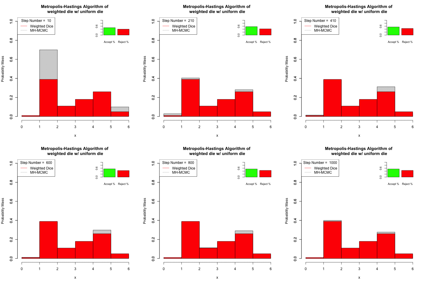
Use the Metropolis-Hastings algorithm to sample from a weighted-die with the distribution

1	2	3	4	5	6
0.01	0.39	0.11	0.18	0.26	0.05

Using an even die, as the proposal step.

The stationary distribution is obviously, $\boldsymbol{\pi} = (0.01,0.39,0.11,0.18,0.26,0.05)$ and the transition matrix, $\boldsymbol{T}$ , is the roll of a fair die. The transition matrix in this case is uniform, i.e. $T_{ij} = \frac{1}{6}$ for all $i$ and $j$ . The equation for acceptance function (1) then simply becomes,

$\begin{equation*}\label{eq:dice} a(i,j) = \frac{\pi_j}{\pi_i} \end{equation*}$

The problem can be easily implemented using your favorite programming language. The following is a solution in R.

The simulated Markov chain converges to the stationary distribution quickly.

Metropolis-Hastings algorithm of a weighted die with stationary distribution(red), and progression of simulated Markov chain(gray).

Continuous space

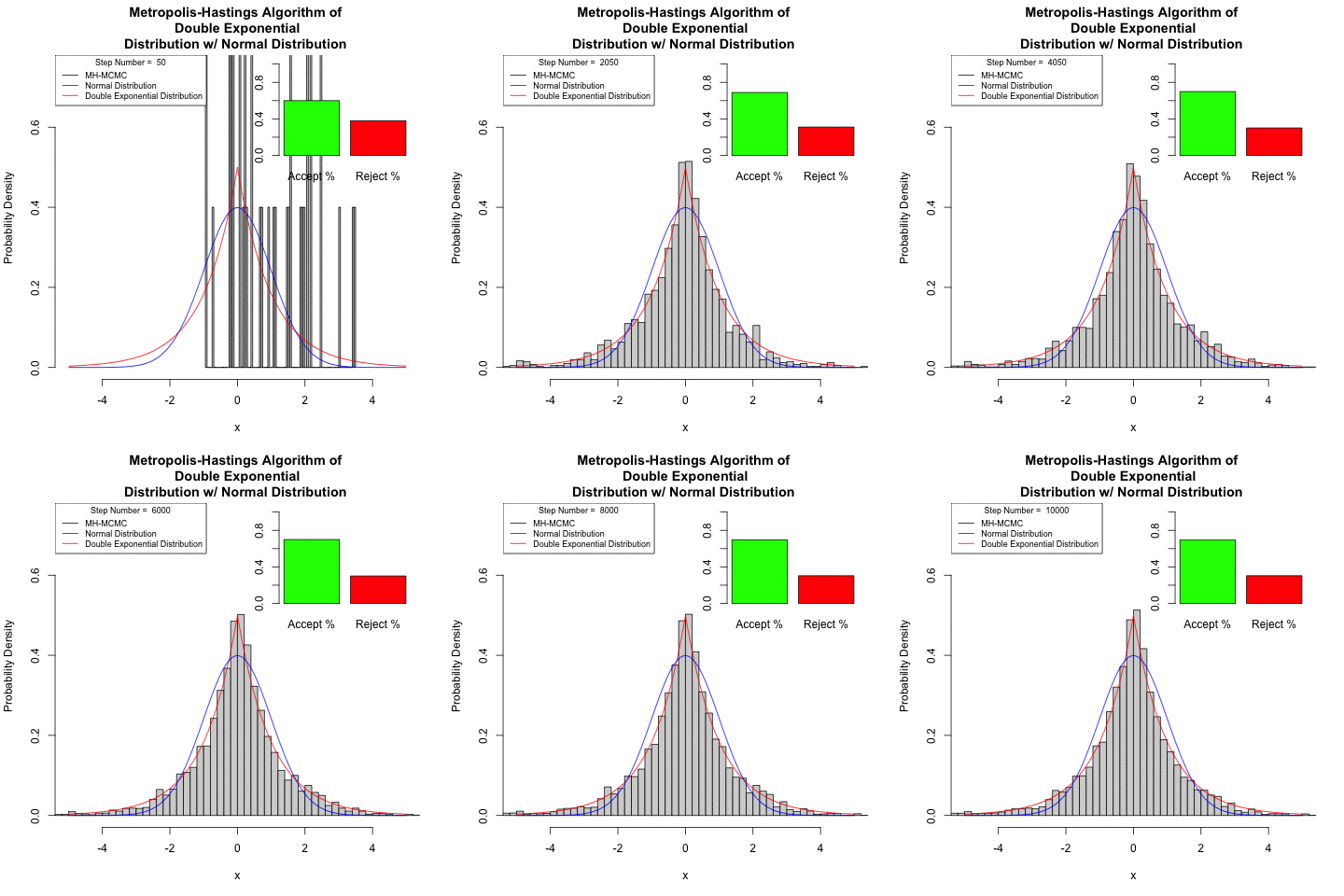
Show how to use the Metropolis–Hastings algorithm to simulate from the double-exponential distribution, with density

$\begin{equation*}\label{eq:double} f(x) = \frac{\lambda}{2} e^{-\lambda |x|},\text{for} \; -\infty < x < \infty \end{equation*}$

The stationary distribution $\pi_t$ is $f(t)$ , from state $s$ , the proposal chain moves to $t$ , where $t$ is normally distributed. The conditional density given $s$ is constant, with

$\begin{equation*}\label{eq:transitiondouble} T_{st} = 1/2, \text{for} \; s - \mathcal{N}(0,1) \leq t \leq s + \mathcal{N}(0,1). \end{equation*}$

The acceptance function is

$\begin{equation*}\label{eq:acceptdouble} a(s,t) = \frac{\pi_t T_{ts}}{\pi_s T_{st}} = \frac{\frac{\lambda}{2} e^{-\lambda |t|} (1/2)}{\frac{\lambda}{2} e^{-\lambda |s|} (1/2)} = e^{-\lambda(|t| - |s|)} \end{equation*}$

Again, the implementation in R

Generally, simulated continuous space Markov chains require more steps for convergence.

Metropolis-Hastings algorithm of the double exponential distribution (red), and progression of simulated Markov chain (gray) using the normal distribution (blue) as a proposal step.

Final Thoughts

These basic examples show the utility of the Metropolis-Hastings algorithm. MH uses an incredibly simple and clear way to solve difficult problems. Those problem, “How do I simulate a difficult distribution, using a simple, well established, distribution?” and “How can cleverly reduce the number of calculations in physical systems?”.